Stochastic models of road traffic

1. Cowan, R. Stochastic properties of equilibrium traffic flow, Ph.D. dissertation UNSW (1970).

2. Cowan, R. A road with no overtaking. Australian Journal of Statistics  13, 2 94-116 (1971).

3. Cowan, R. and Eriksson, S. On the floating vehicle problem. Proc. ARRB. 6, 3 137-143 (1972).

4. Cowan, R. A closed-circuit road. Transportation Research  8, 157-159 (1974) .

5. Cowan, R. A mathematical study of one and two lane roads. Aust. Road Research Board Tech. Report (1974)

6. Cowan, R. Useful Headway Models. Transportation Research  9, 371-375 (1975).

11. Cowan, R. An improved model for signalised intersections with vehicle-actuated control. J. Applied Probability  15, 384-396 (1978).

12. Cowan, R. The uncontrolled traffic merge. J. Applied Probability  16, 384-392 (1979) .

17. Cowan, R. Further results on single-lane traffic flow. J. Applied Probability  17, 523-531 (1980).

18. Cowan, R. Signalised intersections - capacity and timing guide. (R. Ackcelik, J. Luk, editors) (1979).

21. Cowan, R. An analysis of the fixed-cycle traffic light problem. J. Applied Probability  18, 672-683 (1981) .

29. Cowan, R. Adams' Formula Revised. Traffic Engineering & Control  25, 5 272-274 (1984). Download in pdf format

34. Cowan, R. An extension of Tanner's results on uncontrolled intersections. Queueing Systems  1, 249-263 (1987).

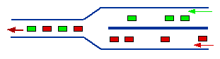
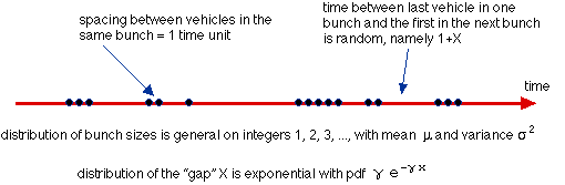
Bunch-gap model: The major theme of this work is the use of a "bunch and gap" arrival model which captures many features of real traffic. The arrival times of vehicles at an intersection or a road entrance (or a place on the road where someone wishes to cross) are assumed to follow this model.

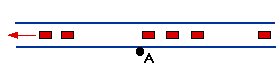
The blue dots on this axis are the times at which the front axle of vehicles cross a line drawn across the road. The temporal spacing between vehicles is called a "headway" and this comprises a "following spacing" plus (if the vehicle is not following its predecessor) a "gap". The flow rate of the traffic per unit time is

.

Note that 0 < λ < 1 and that our "time unit" is the temporal spacing (in practice about 2 seconds) between cars within a bunch. This should not be confused with the flow rate which is usually expressed as vehicles/min in engineering studies and denoted by the symbol q. So their "q" equals 30 times our "λ".

As a sample of the type of problems studied and results available (in papers #11, #12, #17, #21, #29 and #34), we consider three situations.

	A man arrives at point A at an arbitrary time independent of the traffic on the road. He wishes to cross the road but can only do so during large headways in the traffic, namely whenever the gap (or residual gap if he arrives at A during a gap) is > β. What is the average delay experienced? Answer (see #29):
A stream of traffic on a minor road wishes to turn left, joining the major stream. A minor road vehicle, when it reaches the stop line, obeys the same gap-acceptance rule as described above for pedestrians, although now β > 1. When a minor-road vehicle merges, any queueing vehicles on the minor road move up one position in the queue, with a move-up time of 1 time unit. The major road vehicles are not delayed at all. What are the average delays to the minor-road traffic, both in waiting to reach the head of the line and and in waiting to merge once at the stop line? What is the capacity of the intersection? Answer: Explicit formulae are available in #34.
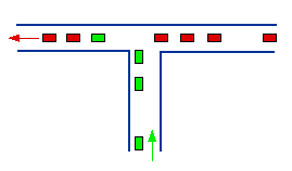n traffic streams merge (here n=2) with no stream having priority over any other. The only constraint is that the cars must wait at the merge point until there is the required one time-unit spacing between themselves and the car in front.	Provided the total flow Λ < 1, then the post-merge traffic stream is a bunch-gap model with gaps being exponentially distributed (parameter Γ) and bunch sizes having mean μ = Λ / Γ(1 - Λ) and variance given (in #12) by Interesting problems in distribution theory arise with the post-merge bunch size (see Thoughts on Borel distribution). The average delay is given by (see #12):

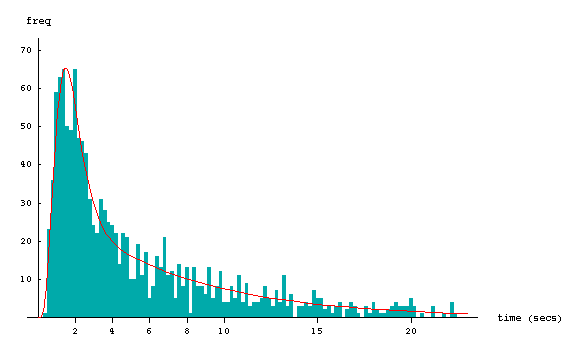
The assumption that the intra-bunch "spacing" (ie "following headway") is exactly one time-unit is relaxed somewhat in #2 and #17. Real point-process data collected on Mona Vale Road in Sydney shows that "following headways" are indeed variable (albeit with low variance relative to that of all headways). These data, presented in #6 and available for download, were stationary (in the point-process sense). The distribution of all headways in the sample of size 1324 is shown below, together with a fitted mixture distribution

which captures the concept that a proportion ψ of cars are following their predecessor at a headway distributed with pdf g whilst the others are not following and therefore leave a "following headway" plus the exponentially distributed gap of our model (that is, the convolution of g and an exponential density).

Various sensible choices of g, namely gamma, inverse Gaussian or lognormal, are fitted below using ML estimation. All three gave excellent fits, there being little to discriminate between them.

The red curve shows the gamma version for g used in the pdf f, plotted against the Mona Vale Road data. I believe that the mixed nature of the distribution is an essential feature behind the excellent fit.

Variance-to-mean ratio of traffic counts

The Poisson process, used as a model when traffic is very light, has the property that the variance of counts in time intervals of length T, divided by the mean of such counts, equals 1. Traffic engineers sometimes calculate this ratio from traffic samples.

For my bunch-gap model, I calculated back in 1979 (though have never published) that, as T gets large, this ratio tends to

.

This formula, derived by Tauberian arguments, gives a reasonable approximation for T > 10 (say) and would certainly work well for practical time intervals of (say) one minute.

Thoughts on the Borel distribution

A random variable M with the Borel distribution on {1, 2, 3, ...} has pmf

If the pgf of M is denoted by Q, then the functional equation Q(z) = z exp[λ(Q(z) - 1)] holds. Also E(M) = 1/(1 - λ) whilst Var(M) = λ/(1 - λ)³.  

Borel showed in 1943 that the number of customers served during the busy period in an M/D/1 queueing system has the distribution above. Thus the times of customers entering service in the M/D/1 system, with arrival rate of λ<1 and service time of one time-unit, is a "bunch-gap" point process of the type shown above in my road traffic work. It has the special properties, though, that (a) bunch sizes have the Borel distribution and (b) Γ = λ. If (a) and (b) hold, I call my bunch-gap process a "Borel point process".

Now if two of these Borel point processes become inputs to the two roads shown in my merging diagram above, then it is an interesting fact that the post-merge process is a Borel point process too. This is readily seen by noting that the post-merge process is the same if the M/D/1 spacing of the Poisson traffic occurs not at the start of the two roads but at the instant before the two streams merge.

Since writing #12, I have derived a set of functional equations for the pgf H (say) of the post-merge bunch in terms of the individual properties of the n arrival streams. For n = 2, and using colour codes for the parameters, H(z) = [γ G(z) + γ R(z) ] / (γ + γ) where G and R are (respectively) the pgf's for post-merge bunches given that the first car in the post-merge bunch is green or red. G and R satisfy jointly the equations

where the coloured H functions are the bunch-size pgf's for the two input streams. Example solutions of (#) are:

Thus, in some cases, there is invariance of the Borel distribution under the merging of traffic streams.

In 2000, I solved (#) for the general case of Borel input bunches. An interesting generalised-Borel distribution arises as the bunch-size distribution in the output stream, namely P{M = m} equal to

where ξ = (μ - 1) / μ within each colour code. When γ = ξ and γ = ξ , whereby the input streams become Borel processes, we retrieve the usual Borel distribution. Likewise, if γ = γ and ξ =ξ, whereby the input streams have identical stochastic structure (with Borel bunches but not necessarily Borel processes), we also get a Borel distribution (though this is not immediately apparent). Furthermore, taking limits as ξ and ξ tend to zero generalises the result above for input bunches of size 1 (encouraging us to think of the constant 1 as a Borel-distributed variate with mean μ = 1).